Variable Rate. We've been hearing about Variable Rate Fertilizer for the last 25+ years. It all starts with an Equation. However, how would you define it? Here's one way to define it:
Equations?!?! Series of conditions??!?!?!

Let's make this easier to understand, but not pretend that equations are simple in agronomic nature.
It really is just taking known pieces of information, or Attributes, and the values associated with them, and manipulating them to accomplish a goal.
Before we look at the evolution of equations, let's understand how to read equations. Learning to read them will help you to understand more and have confidence in explaining your recommendation.

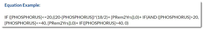
This equation is calling for any soil test Phosphorus values under 30 ppm to apply a build rate.
However, you cannot build soil test levels without putting on a removal rate. These removals can be based off of a yield goal or actual removed calculated from the yield file. They look something like this:

The ([YieldGoalCorn]*.38) is an example of a yield goal and the removal value is 0.38# P2O5/bu. 0.38 is a value set by the user. Your removal value may differ.
The [PRem] is an example of a calculated removal from a yield file that has already been calculated in PCS.
Let's put it all together and test your knowledge!


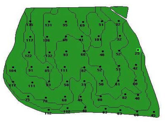
Level 1: Early Equations were designed to make the map 1 color. Mine the high areas and build up the low areas.
Pros:
- Better than whole field spread (flat rate).
- Attempts to account for crop removals.
- The yield goals can be adjusted to individual growers average yields.
Cons:
- The yield goals are a field average or yields the same.
- Does not account for productivity zones.
Level 2: Spatial Yield Goal
This type uses actual yield by soil type data to define spatial yield goals.
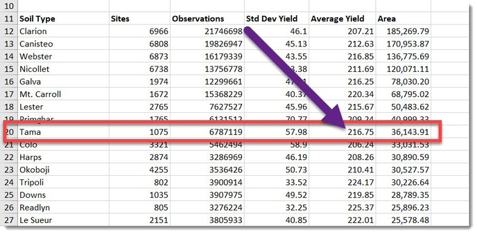
With a deep database, you can use the query tool to define yield goals by soil type. For this example, you can see where Tama soil's average yield has been 216.75 bu/acre and other soil types in this group vary from it.
Pros:
- Better than whole field yield goals.
- Soil types do have some correlation to yield.
Cons:
- Soil type does not always match yield.
- Does not account for productivity zones.
Level 3: Actual Crop Removals
This type uses a yield file allows for accounting for removal of nutrients at an even more precise level.
Pros:
- Ability to incorporate what was removed by the crop spatially.
- Growers can see the yield changes on their monitor and want to replace nutrient rates accordingly.
Cons:
- Does not account for productivity zones.
- Leaves Grower vulnerable to building fertility where a higher return is not possible.
Let's look at another equation to see the difference!
Going Beyond Level 3 - Response Curves
A response curve tells us that at the lower fertility ranges there is a higher chance of a response to added fertilizer and the response is also larger.
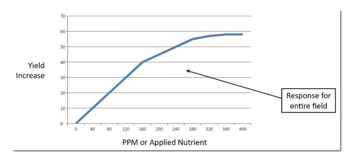
Higher Productive areas have higher response.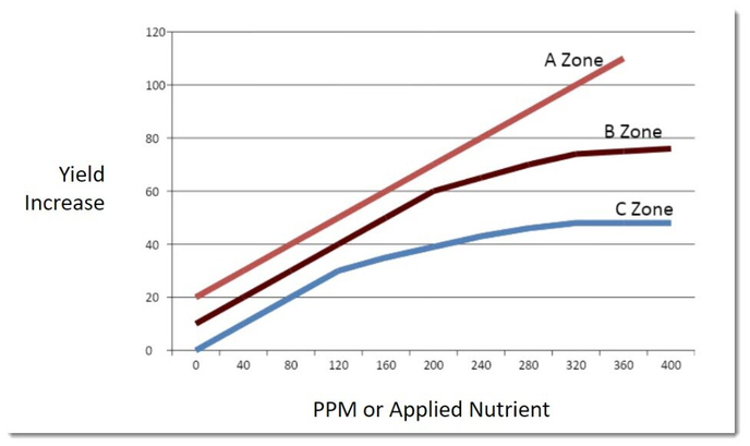
Conclusions:
- If you combine the A,B,C zones you will get the traditional curve. It is just like taking a composite soil sample from a field.
- If you look at each zone separately you will see that the A Zone doesn’t flatten out and continues to provide a high ROI while the C Zone levels off due to other factors like moisture.
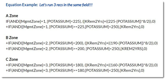
Level 4: Incorporating Zone Management
Why Management Zones?
- Historic yield data shows areas that consistently yield higher
- Manage those areas independently (fertilizer, etc.)
- Doesn't compromise the agronomy
- A zones provide a high ROI
- C zones have other yield limiting factors - do we need to build fertility as high?

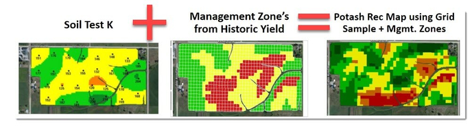
Doesn't it make more sense? Doesn't it look more complex? But, it was easy to create!
You don't have to be an expert at equations, as we're here to assist you, but understanding how to read the equation can help you become a better advisor.